Quick Start Instructions
Install PGL
To install Paddle Graph Learning, we need the following packages.
paddlepaddle >= 2.0.0
cython
We can simply install pgl by pip.
pip install pgl
Introduction
Paddle Graph Learning (PGL) is an efficient and flexible graph learning framework based on PaddlePaddle.
To let users get started quickly, the main purpose of this tutorial is:
Understand how a graph network is calculated based on PGL.
Use PGL to implement a simple graph neural network model, which is used to classify the nodes in the graph.
Step 1: using PGL to create a graph
Suppose we have a graph with 10 nodes and 14 edges as shown in the following figure:
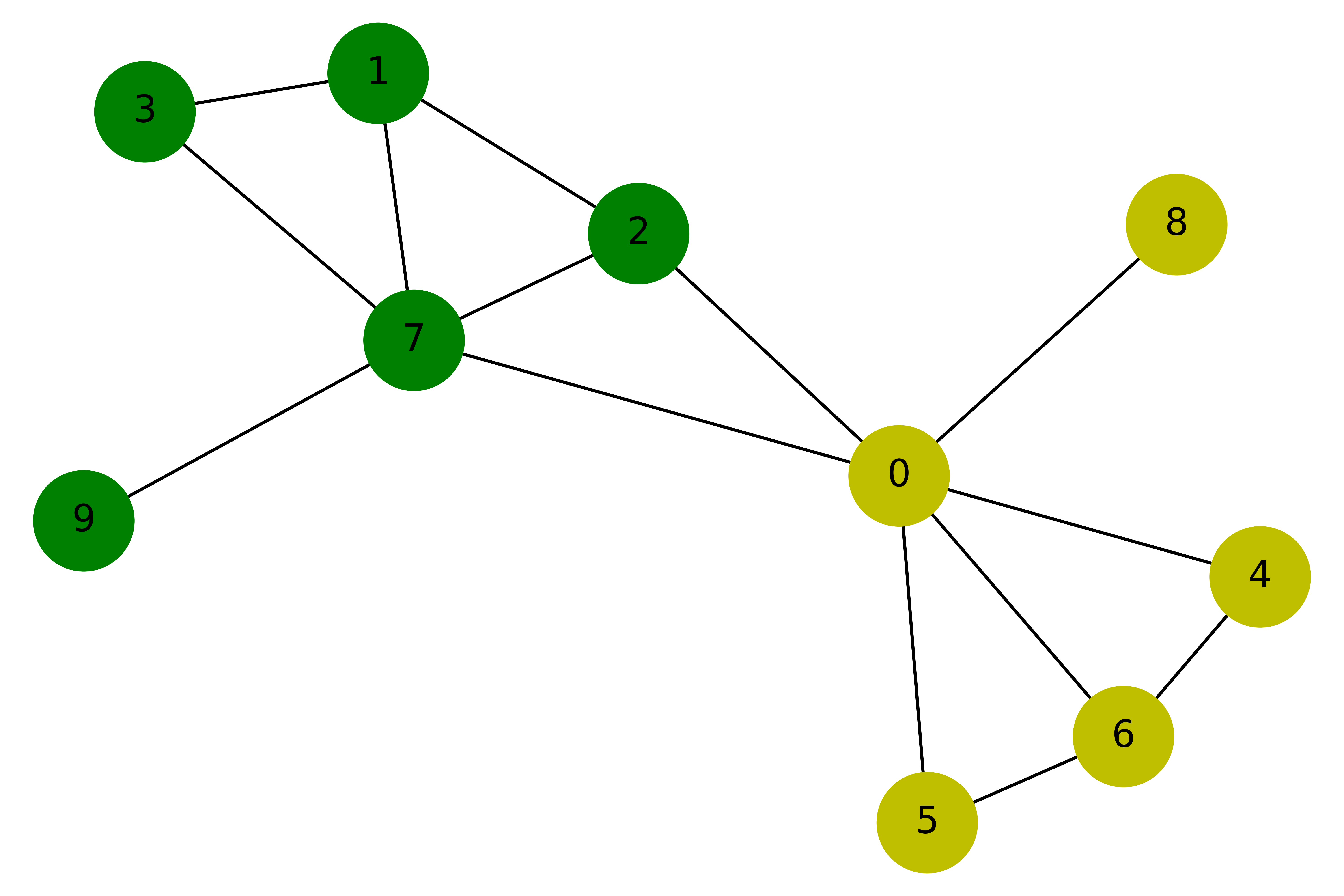
Our purpose is to train a graph neural network to classify yellow and green nodes. So we can create this graph in such way:
import numpy as np

import paddle
import paddle.nn as nn
import paddle.nn.functional as F
from paddle.optimizer import Adam
import pgl


def build_graph():
    # define the number of nodes; we can use number to represent every node
    num_node = 10
    # add edges, we represent all edges as a list of tuple (src, dst)
    edge_list = [(2, 0), (2, 1), (3, 1),(4, 0), (5, 0),
             (6, 0), (6, 4), (6, 5), (7, 0), (7, 1),
             (7, 2), (7, 3), (8, 0), (9, 7)]

    # Each node can be represented by a d-dimensional feature vector, here for simple, the feature vectors are randomly generated.
    d = 16
    feature = np.random.randn(num_node, d).astype("float32")
    # each edge has it own weight
    edge_feature = np.random.randn(len(edge_list), 1).astype("float32")

    # create a graph
    g = pgl.Graph(edges = edge_list,
                  num_nodes = num_node,
                  node_feat = {'nfeat':feature},
                  edge_feat ={'efeat': edge_feature})

    return g
g = build_graph()
After creating a graph in PGL, we can print out some information in the graph.
print('There are %d nodes in the graph.'%g.num_nodes)
print('There are %d edges in the graph.'%g.num_edges)
There are 10 nodes in the graph.
There are 14 edges in the graph.
Step 2: create a simple Graph Convolutional Network(GCN)
In this tutorial, we use a simple Graph Convolutional Network(GCN) developed by Kipf and Welling to perform node classification. Here we use the simplest GCN structure. If you want to know more about GCN, you can refer to the original paper.
In layer \(l\),each node \(u_i^l\) has a feature vector \(h_i^l\);
In every layer, the idea of GCN is that the feature vector \(h_i^{l+1}\) of each node \(u_i^{l+1}\) in the next layer are obtained by weighting the feature vectors of all the neighboring nodes and then go through a non-linear transformation.
In PGL, we can easily implement a GCN layer as follows:
class GCN(nn.Layer):
    """Implement of GCN
    """

    def __init__(self,
                 input_size,
                 num_class,
                 num_layers=2,
                 hidden_size=16,
                 **kwargs):
        super(GCN, self).__init__()
        self.num_class = num_class
        self.num_layers = num_layers
        self.hidden_size = hidden_size
        self.gcns = nn.LayerList()
        for i in range(self.num_layers):
            if i == 0:
                self.gcns.append(
                    pgl.nn.GCNConv(
                        input_size,
                        self.hidden_size,
                        activation="relu",
                        norm=True))
            else:
                self.gcns.append(
                    pgl.nn.GCNConv(
                        self.hidden_size,
                        self.hidden_size,
                        activation="relu",
                        norm=True))

        self.output = nn.Linear(self.hidden_size, self.num_class)
    def forward(self, graph, feature):
        for m in self.gcns:
            feature = m(graph, feature)
        logits = self.output(feature)
        return logits
Step 3: data preprocessing
Since we implement a node binary classifier, we can use 0 and 1 to represent two classes respectively.
y = [0,1,1,1,0,0,0,1,0,1]
label = np.array(y, dtype="float32")
Step 4: training
The training process of GCN is the same as that of other paddle-based models.
g = g.tensor()
y = paddle.to_tensor(y)
gcn = GCN(16, 2)
criterion = paddle.nn.loss.CrossEntropyLoss()
optim = Adam(learning_rate=0.01,
             parameters=gcn.parameters())
gcn.train()
for epoch in range(30):
    logits = gcn(g, g.node_feat['nfeat'])
    loss = criterion(logits, y)
    loss.backward()
    optim.step()
    optim.clear_grad()
    print("epoch: %s | loss: %.4f" % (epoch, loss.numpy()[0]))
epoch: 0 | loss: 0.7915
epoch: 1 | loss: 0.6991
epoch: 2 | loss: 0.6377
epoch: 3 | loss: 0.6056
epoch: 4 | loss: 0.5844
epoch: 5 | loss: 0.5643
epoch: 6 | loss: 0.5431
epoch: 7 | loss: 0.5214
epoch: 8 | loss: 0.5001
epoch: 9 | loss: 0.4812
epoch: 10 | loss: 0.4683
epoch: 11 | loss: 0.4565
epoch: 12 | loss: 0.4449
epoch: 13 | loss: 0.4343
epoch: 14 | loss: 0.4248
epoch: 15 | loss: 0.4159
epoch: 16 | loss: 0.4081
epoch: 17 | loss: 0.4016
epoch: 18 | loss: 0.3963
epoch: 19 | loss: 0.3922
epoch: 20 | loss: 0.3892
epoch: 21 | loss: 0.3869
epoch: 22 | loss: 0.3854
epoch: 23 | loss: 0.3845
epoch: 24 | loss: 0.3839
epoch: 25 | loss: 0.3837
epoch: 26 | loss: 0.3838
epoch: 27 | loss: 0.3840
epoch: 28 | loss: 0.3843
epoch: 29 | loss: 0.3846